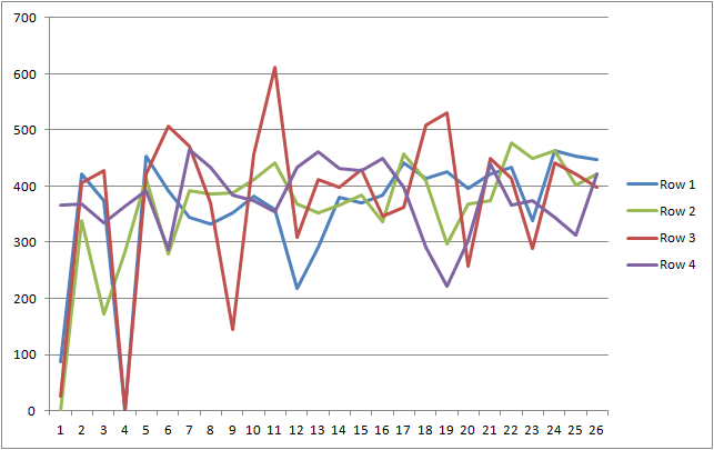
Overview

Back EMF speed control operates by monitoring the induced back EMF created by the motor windings turning within the motor’s static magnetic field.
This back EMF is directly proportional to motor speed.

By regularly interrupting the PWM drive to the motor, the back EMF voltage can be measured and used to adjust the PWM drive to maintain a nominally constant speed.

Implementation

The timing for BEMF control is based upon 128 counts @ a 131us interval.
Drive is present for 100 counts, and absent for the remaining 28.
ie, the typical the BEMF sampling interval lasts for ~3.7ms of a 16.8ms period.

The original loco decoder code takes a single ADC sample half way through this 3.7ms dead time.
This basic method is very prone to sampling noise such as commutation segments and dirty brushes.

It has been suggested that taking several ADC samples during the sample interval and performing a median average could produce a more stable feedback term into the BEMF algorithm.

Sampling Analysis

To test the concept, I adapted my Development Board software to take ADC samples every 131 us during the sampling interval. (using the same timebase for the BEMF control)
This results in 26 samples within the 3.7ms interval.

For analysis on a PC, the fresh 10 bit ADC values are immediately sent over the RS232 port and captured to a file.
RS232 @ 115200 baud can send more than 190 characters during the 16.8ms BEMF period. 26 samples as 3 character HEX values plus a delimiter is just over 100 characters, so no data should be lost due to buffer overrun.

The captured data was then imported into Excel where charting functions can be quickly and easily performed.

The following chart is of the raw ADC samples from 4 consecutive intervals.
Note the earliest samples show the initial negative kick when motor drive is first suspended, these then return to a level indicative of motor speed via the back EMF

The noisy nature of these ADC samples is clearly obvious.

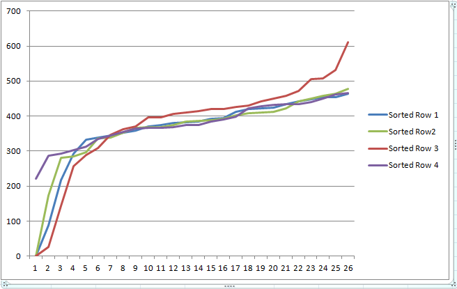
What is most interesting is the chart of these exact same samples after being sorted:

The similarity now between the previously noisy traces is absolutely stunning.
Of particular note is “row 3” which appears very wild in the raw time series.
If one ignores the upper and lower ends of the sorted data, the median values are very consistent. The first samples would be from the initial negative kick as described earlier.

One could simply take the single centre sample (#13) from the sorted data (ala median) and have a much improved estimate than would be derived from the raw time series data around sample 13 (of which sample #12 does appear to be particularly bad).
It truly is quite a stunning result from a simple reordering.

Averaging several of the median ADC readings would provide an even smoother end result.

Excel spreadsheet

28th August 2012.